Modelado de datos en Power BI

En anteriores post vimos como Power BI nos podía ayudar a analizar la información de nuestra cadena de bocadillos. Pero ¿Cómo llegamos a visualizar la información? Y lo más importante de todo: ¿Cómo hacemos que esta información sea manejable por el usuario? La respuesta siempre reside en la potencia de nuestro modelo.

Teniendo en cuenta el mismo modelo de negocio, nuestra cadena de bocadillos ha crecido y gracias a la ayuda de nuestros nuevos socios franquiciados, se ha expandido por algunas provincias de la península. Estos franquiciados funcionan de diferente manera que las tiendas propias y generan un beneficio a la matriz menor que las tiendas propias. ¿Quién será mejor vendiendo bocadillos, las franquicias o las tiendas propias? Veamos cómo montar el modelo para obtener respuestas.

Para poder realizar este ejemplo, contamos con tres tablas: La primera de ellas es un maestro de artículos; la segunda es maestro de tiendas; la tercera contiene los tickets de las tiendas.

En primer lugar lo que vamos a hacer es importar estas tablas a nuestro Power BI desktop. Recordemos que estás tablas pueden residir en multitud de orígenes de datos. En este caso, todos nuestros datos serán obtenidos desde un Excel.

Lo primero que debemos de hacer es presionar el botón “Get Data” y a continuación seleccionaremos el apartado File > Excel:

Seleccionamos nuestro fichero Excel y a continuación detectará las tablas que tengamos en nuestro Excel. Si los rangos de datos se han formateado como tablas, además de las hojas nos mostrará estas.

Seleccionaremos las tres tablas. Cuando seleccionamos alguna de ellas, en el panel de la derecha, se mostrará una vista previa. Hacemos click en “Load” y cargaremos nuestras tablas al modelo.

A continuación, haremos click en la parte de la izquierda, en el icono de tabla. Allí se mostrarán las tablas que hemos cargado.

A continuación, vamos a establecer las relaciones entre las tablas. Si PowerBI detecta nombres de columnas iguales, establece las relaciones entre las tablas. Para ver esta relación vamos al botón de relaciones:

Como vemos, ha relacionado la tabla Ventas con Articulos y con Tiendas. A continuación podemos empezar a establecer cuáles son los tipos de datos para las columnas.

Comenzamos con Ventas:

En las ventas, vemos que ha detectado IDVenta, Ticket y Cantidad como una métrica. Al ser un tipo númerico, PowerBI toma la columna como medible. En este caso, no nos va dar ninguna información sumar el identificador de la venta ni el identificador del ticket. Convertiremos dichas columnas en tipo texto para que no las tome como métrica.

Para hacer este paso, volvemos a la vista de tabla, seleccionamos la columna IDVenta y cambiamos el tipo a “Text”:

Repetimos el mismo paso para Ticket. Además, podemos apreciar que no tenemos precios de venta en la tabla de ventas. Vamos a utilizar formulas DAX para obtener el dato (que reside en la tabla Articulos). DAX es un lenguaje de expresiones que nos va a permitir realizar diferentes cálculos. Este lenguaje, aunque tiene una sintaxis parecida al lenguaje de formulas de Excel, es mucho más complejo y está orientado a la realización de cálculos complejos. Hablaremos de él en próximos posts.

Para recuperar los precios, realizaremos lo siguiente. Crearemos una nueva columna en la que pondremos las siguiente fórmula.

RELATED (Articulos[PVP)

Related busca una columna en otra tabla relacionada. Al haber una relación puede traer la columna como lo podríamos hacer con un BUSCARV en Excel.
Repetimos la misma operación para las columnas Articulos[PVP Franquiciado] y Tiendas[Es Franquicia]. Renombramos las columnas haciendo click derecho sobre ellas > Rename y les ponemos nombre que los identifique correctamente.

El resultado es el siguiente:

A continuación, vamos a definir el PVP que tenemos que utilizar. Si la tienda es Franquicia, utilizaremos PVP franquicia y si no, utilizaremos PVP. Introducimos una nueva columna con la siguiente fórmula:

PVP Final = IF(Ventas[Es Franquicia]=”Si”;Ventas[PVP Franquicia];Ventas[PVP])

Crearemos otra columna con la venta, que será el PVP Final * Cantidad:

Venta = Ventas[PVP Final]*Ventas[Cantidad]

Una columna, que si es pago con tarjeta, perderemos un 0,01% de la venta en concepto de comisiones:

Comision Tarjeta = Ventas[Venta]*0,01

Obtendremos también los beneficios que se obtienen por producto y, como hemos hecho en con los PVP, obtendremos cual obtener.

Beneficio = RELATED(Articulos[Beneficio])-Ventas[Comision Tarjeta]

Beneficio a matriz = IF(Ventas[Es Franquicia]=”Si”;RELATED(Articulos[Beneficio Franquiciado])*Ventas[Venta];0)

Beneficio Tienda Final = IF(Ventas[Es Franquicia]=”Si”;Ventas[Beneficio]-Ventas[Beneficio a matriz];Ventas[Beneficio])

A continuación, esconderemos las columnas que no necesite el usuario. Estás serían los identificadores que tenemos en la tabla de Ventas y las columnas auxiliares que hemos recuperado. Para esconder una columnas, hacemos click en la cabecera > Hide in Report View. El resultado obtenido es el siguiente (en gris las columnas escondidas):

Por último crearemos las métricas.

Para crear una métrica, tenemos que hacer click en el botón “Create Measure” y escribir la fórmula de la nueva métrica.

Crearemos las siguientes métricas:

Numero de Tickets = DISTINCTCOUNT([Ticket])

Total de Ventas = SUM(Ventas[Venta])

Beneficio Matriz = SUM(Ventas[Beneficio a matriz])

Beneficio Tienda = SUM([Beneficio Tienda Final])
Creadas las métricas, vamos a la vista de Reporte. En la parte de la derecha podemos ver los campos disponibles para el usuario. Hay que hacer notar que es importante eliminar aquellos campos que no nos van a aportar o que son repetitivos.

Ahora jugando un poco con los campos podemos hacer cosas como estas:

En este post hemos visto como:

• Es importante trabajar el modelo. No nos debemos de limitar a tener una sola tabla con todo junto. Separemos las diferentes entidades y apoyémonos en ellas para obtener los datos que necesitamos para el análisis.
• Establezcamos los tipos de datos correctos. Nunca sumariamos dos números de teléfono, al igual que la suma de dos identificadores no nos aporta nada.
• Dejemos disponibles solo aquellos datos que son relevantes para el análisis. Escondamos identificadores o columnas recurrentes
• Convirtamos aquellas columnas de datos en métricas. Ayudará al usuario a saber qué columnas se pueden medir.

Modelado Avanzado de datos y Calculos usando Power BI

Power BI Model Size Bloat And Auto Date/Time Tables

Opinion is split over Power BI’s ability to automatically create Date hierarchies in your model. Personally it drives me mad and I always turn it off, but I know a lot of people love the convenience of it. Whatever your feelings, though, it is important to be aware of the problems it can cause with the size of your model.

Imagine you have a .pbix file and you load just this one table into the data model:

 

Three columns, each containing three dates with long gaps in between, but only nine values overall. No other tables or queries, no measures, no visuals at all. When you save it results in a file that is a massive 4.7MB – but why, when there’s hardly any data?

Actually, there is a lot of data hidden in this file. If you connect to the .pbix file with DAX Studio you can see that the Auto Date/Time functionality has built three hidden Date tables whose names are prefixed with “LocalDateTable”, one for each date column in the original table above:

 

These tables can be queried in DAX Studio, and the following query reveals more about them (if you try this on your model you will need to alter the name of the table used in the query to match the names of one of the tables in your model):

1

2

3

4

5

6

7

8

9


EVALUATE

ROW (

"Hidden Date Table Rowcount", 

COUNTROWS ( 'LocalDateTable_17eac8aa-f559-4ade-971f-9a1ad5258fbe' ),

"Min Date", 

MIN ( 'LocalDateTable_17eac8aa-f559-4ade-971f-9a1ad5258fbe'[Date] ),

"Max Date", 

MAX ( 'LocalDateTable_17eac8aa-f559-4ade-971f-9a1ad5258fbe'[Date] )

)

In this case each of the three tables has 109938 rows. That’s one row for each date between the beginning of the year containing the earliest date in the source column and the end of the year containing the latest date in the source column – which is the best practice for building a Date table, but results in three very large tables in this case.

To stop Power BI automatically building these tables for you, in Power BI Desktop go to the File menu, select Options, then Data Load and deselect the Auto Date/Time option:

When you do this the automatically created date tables are removed from the model. In this case, after saving, the .pbix file shrinks to 181KB! Remember that, by doing this, you won’t get automatic date hierarchies created for you when you are designing your reports and you will have to build any Date tables and hierarchies you need manually.

This is an extreme example of course, but overall you should probably turn off Auto Date/Time if your model size is an issue and:

• You have a lot of date columns in your tables, or
• Your date columns contain large ranges of dates. Remember that some systems use 1/1/1900 as an ‘unknown’ date value, which can make things a lot worse.

Construir tablas de datos desde cero Porwe Bi

Custom Date Tables

Recently at work I’ve been working with a number of large data warehouses with time series data.  Often when working on such data you need to incorporate a data calendar to compute date ranges.  So, for this tutorial we will build a custom date table directly inside PowerBI.

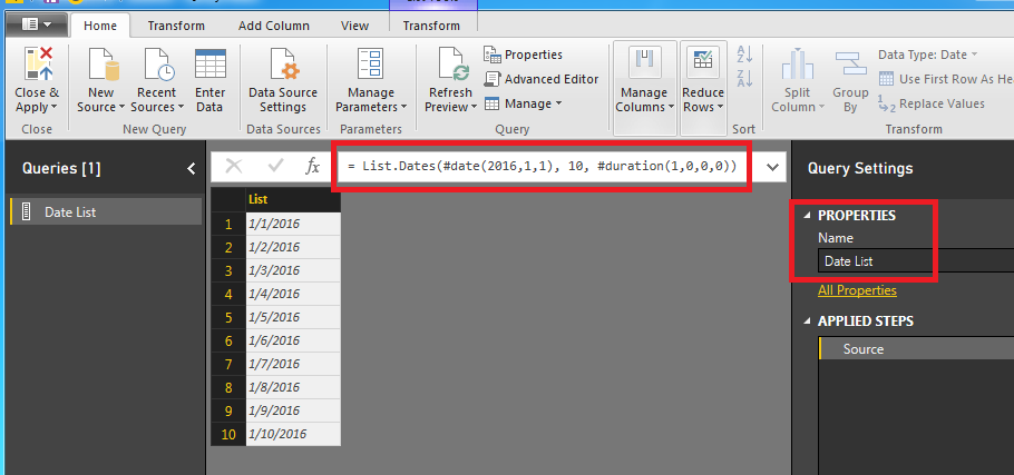
Start by opening up power BI and clicking Get Data on the home ribbon, then select Blank Query.  Like always make sure you start by re-naming the query into something meaningful.  Change the name of the Query to Date List.  Next enter the following equation into the formula bar:

List.Dates( #date(2016,1,1), 10, #duration(1,0,0,0))

Note:  For more information on the M language you can visit here.  Also, here is the link to the List.Dates function found here.

Once we enter the formula into the formula bar the list of dates will appear below.

Date List

The quick explanation about the List.Dates function is below.  I’ve simplified the variables below:

List.Dates(  Start Date  ,   Number of intervals   ,  Type of interval  )

While this is interesting it does not help us make a report that updates the date range dynamically.  The real world use case for this would be you have a report with data that is being generated daily, say for example a website.  Maybe you want a custom date range that automatically changes every day you log into PowerBI.  For example if today is 08-20-2016, I want the first date to be today and then list the dates that previous 10 days.

Now change the formula to the following formula:

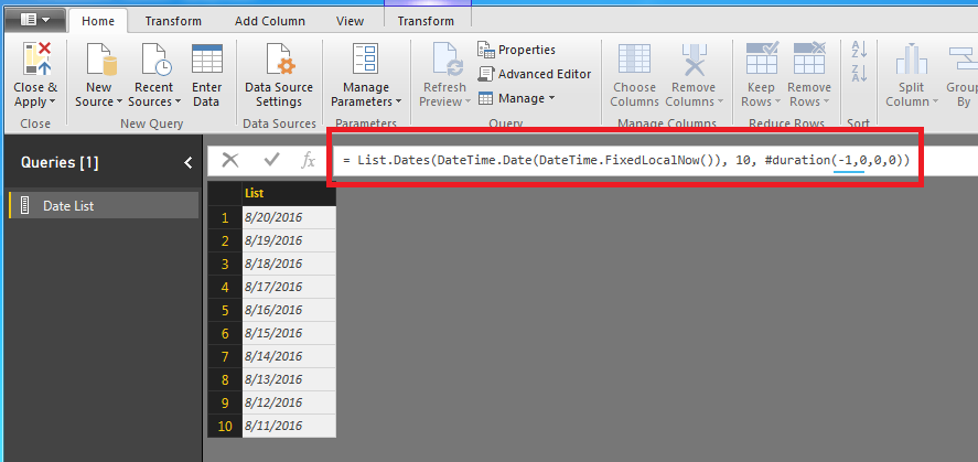
= List.Dates(  DateTime.Date(  DateTime.FixedLocalNow() ) ,  10 ,  #duration(-1,0,0,0)  )

Note:  In this equation we have changed the duration to -1.  This is important to note because now our date table returns older dates.  In our previous equation we used a positive 1 and we return future dates.

In this new equation we have defined the Start Date to the following statement : DateTime.Date(  DateTime.FixedLocalNow() )  This is tricky because if you only use DateTime.FixedLocalNow() the statement will error out.  The error occurs because the DateTime.FixedLoaclNow() is a date and time.  The List.Dates function is expecting a Date only value.  Hence why we use the DateTime.Date() function to remove the time stamp and only return today’s date.

Date List Using Date of Today

It is most likely your date ranges will be different than the ones in the example because the DateTime.FixedLocalNow() function will be pulling in your computer’s current date.

Next modify the equation to now pull the last 90 days (highlighted in red below)

List.Dates(DateTime.Date(DateTime.FixedLocalNow()), 90, #duration(-1,0,0,0))

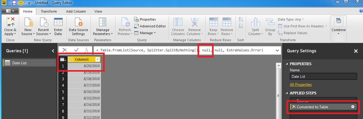
The list of dates is just that a list.  We really can’t do to many other enhancements to our data with only a list of dates.  Now transform the list into a table.  Click on the Transform ribbon and select To Table.  Notice now that we have a new column and a new applied step.

New Column

The code for the new applied steps is as follows:

Table.FromList(Source , Splitter.SplitByNothing() , null , null , ExtraValues.Error)

I colored the first null in the equation.  This is actually a parameter that you can use to name the new column we just made.  Tricky, Tricky, PowerBI.  Modify the equation to the following:

Table.FromList(Source , Splitter.SplitByNothing() , {"Date"} , null, ExtraValues.Error)

Our table is updated and now has the name Date.  Nice work!

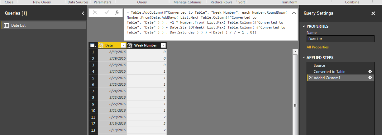
Now lets make our date list useful.  Click on the ribbon labeled Add Column and then the button labeled Add Custom Column.  Add the following equation to the new column and name it Week #, then click OK, to continue.

Number.RoundDown( Number.From(Date.AddDays( List.Max( Table.Column(#"Converted to Table", "Date" ) ) , -1 * Number.From( List.Max( Table.Column(#"Converted to Table", "Date" ) ) - Date.StartOfWeek( List.Max( Table.Column( #"Converted to Table", "Date" ) ) , Day.Saturday ) ) ) -[Date] ) / 7 + 1 , 0)

This equation defines the start of the week highlighted in RED.  Since today is Tuesday 8/30/16, then the days 8/30 (Tues), 8/29 (Mon), 8/27 (Sunday) are considered week 0 or the current week.  All dates prior will start with weekly increment.

Date List

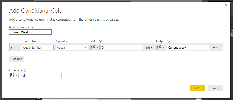
Now we can add some logic to define week variables.  Click on the Add Column ribbon and select the Conditional Column button.  Using the drop downs in Column Name, Operator, Value and Output enter the following:

Current Week Logic

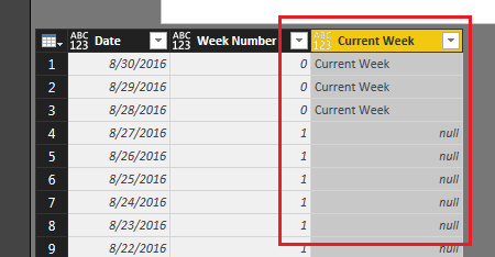
Click OK to proceed.  We have now added an additional column with a text description of the week.

Current Week Column

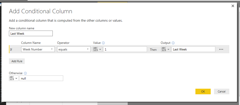
Following the add column steps mentioned above we will now add more week descriptions.  Add the following conditional column for Last Week:

Last Week Logic

From here you can make custom columns for how you want to describe your data.  In this example we will build last 2 weeks, 3 weeks and last 4 weeks.  See the add conditional column logic for each of those respective weeks.

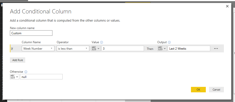
Conditional Column Logic for last 2 weeks:

Last 2 Weeks Logic

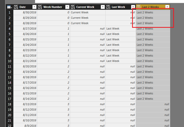
Note: When we added this conditional column we label week 0 as last 2 weeks.  See image below as an example:

Last 2 Weeks Column

To fix this we modify the code that generated this column.  The code initially states the following:

= Table.AddColumn(#"Added Conditional Column1", "Last 2 Weeks", each if [Week Number] < 3 then "Last 2 Weeks" else null )

We modify this code to the following: (changes highlighted in bold)

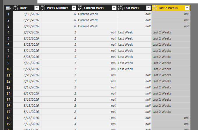
= Table.AddColumn(#"Added Conditional Column1", "Last 2 Weeks", each if [Week Number] < 3 and [Week Number] > 0 then "Last 2 Weeks" else null )

This now removes the first three days from our Last 2 Weeks column reflecting a more accurate picture of our time ranges.

Corrected Last 2 Weeks Column

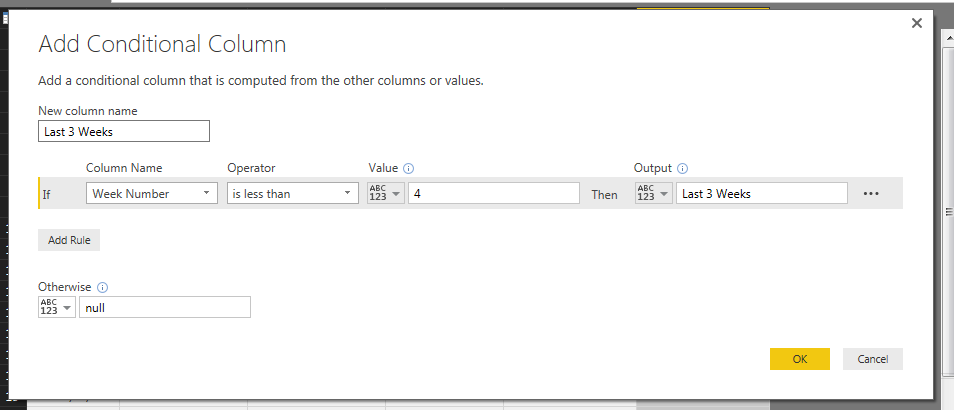
Next we will add the Last 3 Weeks column and the Last 4 weeks column.  Each time we will modify the add column code to remove the first three dates of the current week.

Last 3 Weeks Logic

Last 3 Weeks auto generated code:

= Table.AddColumn(#"Added Conditional Column2", "Last 3 Weeks", each if [Week Number] < 4 then "Last 3 Weeks" else null )

We modify to the following to achieve the correct Last 3 Weeks data range: (changes highlighted in bold)

= Table.AddColumn(#"Added Conditional Column2", "Last 3 Weeks", each if [Week Number] < 4 and [Week Number] > 0 then "Last 3 Weeks" else null )

Add the Last 4 Weeks column:

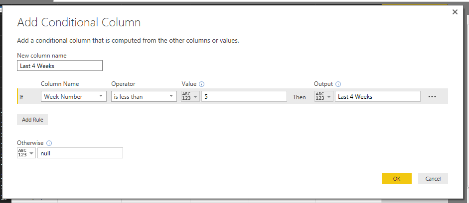
Last 4 Weeks Logic

Last 4 Weeks auto generated code:

= Table.AddColumn(#"Added Conditional Column3", "Last 4 Weeks", each if [Week Number] < 5 then "Last 4 Weeks" else null )

Modify the code the following to correct the column: (changes highlighted in bold)

= Table.AddColumn(#"Added Conditional Column3", "Last 4 Weeks", each if [Week Number] < 5 and [Week Number] > 0 then "Last 4 Weeks" else null )

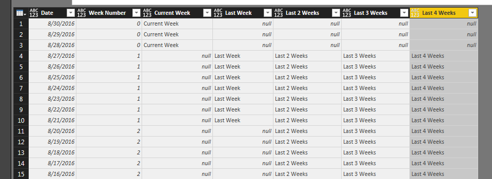
Nice job so far.  We are almost to the end now.  After all those additional columns you should have something that looks similar to the following:

Date Table

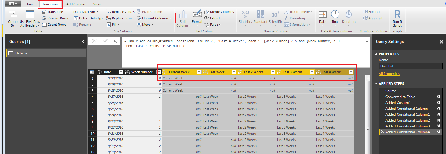
Next we will pivot all the data down to one column.  This will enable us to select a time period and automatically have our date table update to the specific range.

First, shift select the following columns, Current Week, Last Week, Last 2 Weeks, Last 3 Weeks, and Last 4 Weeks.  Then on the Transform ribbon click the Unpivot Columns button.

Unpivot Columns Command

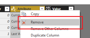
Next delete the Attribute column using a right click on the Attribute column and selecting Remove Columns.

Remove Attribute Column

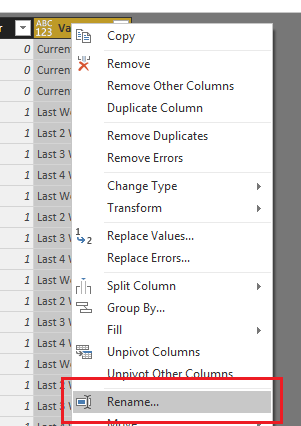
Rename the Value column to Selector by right clicking on the Value column.

Rename the Value Column

Modify each column to have the correct Data Type on the Home ribbon.

Date column data type should be Date

Week Number column data type should be Whole Number

Selector column data type should be Text

Note: It is important to always check your data types for each column before you leave the Query Editor.  If you don’t you’ll find that the visuals that your trying to build later on on the page view will not work as expected.

Next, click the Home ribbon and select Close & Apply.  You can now build the following visuals:

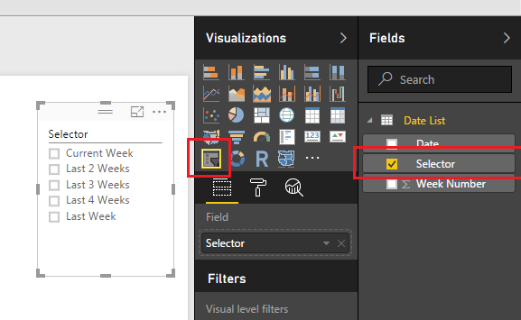
A slicer for the Selector column:

Selector Column as a Slicer

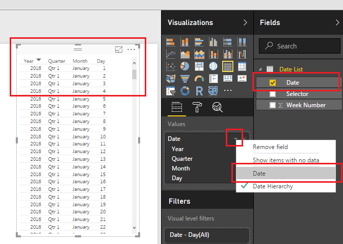
Table visual for the Date column:

Note: When you use the Date Column as the data source for the Table Visual the data will automatically be added as a Date Hierachy.  This does not work well with our data so you will need to change the date from a Date Hierarchy to a standard Date.  To do this click the little triangle next to the Date in the Values box.  Then select Date.

Date Table

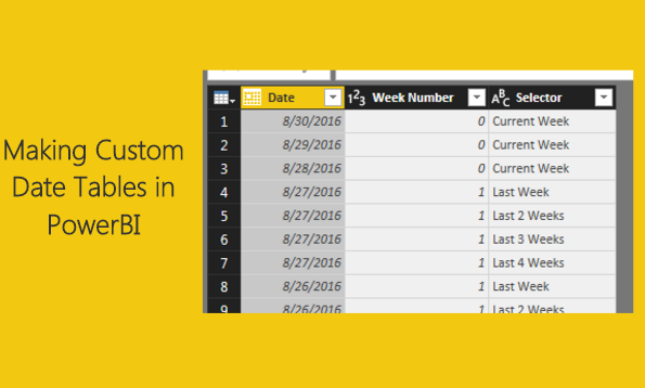
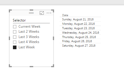
Now you can finally play around with your data and by selecting different items in the Selector slicer you can filter down to different date ranges.  Below I selected the Last Week item, which filters down my dates to only the 7 days from last week.

Last Week Slicer Selected

Nice job making a custom date table in PowerBI.  The nice part about this table is that it will always refresh with the latest dates whenever the queries are refreshed for this PowerBI file.

Bonus:  For those of you who want to cheat and just have the M code to generate this custom date table it can be used from here:

let
 Source = List.Dates(DateTime.Date(DateTime.FixedLocalNow()), 90, #duration(-1,0,0,0)),
 #"Converted to Table" = Table.FromList(Source, Splitter.SplitByNothing(), {"Date"}, null, ExtraValues.Error),
 #"Added Custom1" = Table.AddColumn(#"Converted to Table", "Week Number", each Number.RoundDown( Number.From(Date.AddDays( List.Max( Table.Column(#"Converted to Table", "Date" ) ) , -1 * Number.From( List.Max( Table.Column(#"Converted to Table", "Date" ) ) - Date.StartOfWeek( List.Max( Table.Column( #"Converted to Table", "Date" ) ) , Day.Saturday ) ) ) -[Date] ) / 7 + 1 , 0)),
 #"Added Conditional Column" = Table.AddColumn(#"Added Custom1", "Current Week ", each if [Week Number] = 0 then "Current Week" else null ),
 #"Added Conditional Column1" = Table.AddColumn(#"Added Conditional Column", "Last Week", each if [Week Number] = 1 then "Last Week" else null ),
 #"Added Conditional Column2" = Table.AddColumn(#"Added Conditional Column1", "Last 2 Weeks", each if [Week Number] < 3 and [Week Number] > 0 then "Last 2 Weeks" else null ),
 #"Added Conditional Column3" = Table.AddColumn(#"Added Conditional Column2", "Last 3 Weeks", each if [Week Number] < 4 and [Week Number] >0 then "Last 3 Weeks" else null ),
 #"Added Conditional Column4" = Table.AddColumn(#"Added Conditional Column3", "Last 4 Weeks", each if [Week Number] < 5 and [Week Number] > 0 then "Last 4 Weeks" else null ),
 #"Unpivoted Columns" = Table.UnpivotOtherColumns(#"Added Conditional Column4", {"Date", "Week Number"}, "Attribute", "Value"),
 #"Removed Columns" = Table.RemoveColumns(#"Unpivoted Columns",{"Attribute"}),
 #"Renamed Columns" = Table.RenameColumns(#"Removed Columns",{{"Value", "Selector"}}),
 #"Changed Type" = Table.TransformColumnTypes(#"Renamed Columns",{{"Date", type date}, {"Week Number", Int64.Type}, {"Selector", type text}})
in
 #"Changed Type"